Top Guidelines Of Excel Formulas

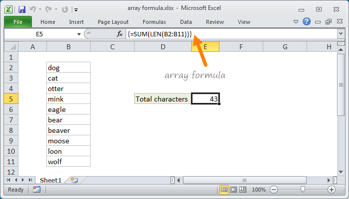
By pushing ctrl+shift+center, this will calculate as well as return value from numerous varieties, instead of simply individual cells added to or increased by each other. Determining the sum, product, or quotient of individual cells is easy-- simply make use of the =SUM formula and also enter the cells, worths, or variety of cells you want to do that arithmetic on.

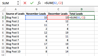
If you're looking to locate total sales earnings from numerous sold systems, for instance, the array formula in Excel is perfect for you. Below's how you would certainly do it: To start utilizing the selection formula, type "=SUM," and also in parentheses, get in the initial of two (or 3, or 4) series of cells you want to increase together.

This stands for multiplication. Following this asterisk, enter your 2nd range of cells. You'll be multiplying this 2nd series of cells by the initial. Your progress in this formula should currently resemble this: =SUM(C 2: C 5 * D 2:D 5) Ready to press Get in? Not so fast ... Because this formula is so complex, Excel gets a various key-board command for selections.

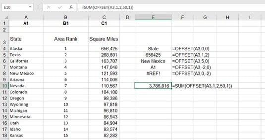
This will certainly acknowledge your formula as an array, covering your formula in support characters as well as successfully returning your product of both ranges combined. In revenue calculations, this can reduce your effort and time significantly. See the last formula in the screenshot above. The MATTER formula in Excel is represented =MATTER(Begin Cell: End Cell).

As an example, if there are eight cells with gotten in worths in between A 1 as well as A 10, =MATTER(A 1: A 10) will return a worth of 8. The MATTER formula in Excel is particularly beneficial for huge spread sheets, where you want to see the number of cells include actual entries. Do not be fooled: This formula will not do any math on the values of the cells themselves.

Learn Excel for Dummies

Utilizing the formula in strong over, you can conveniently run a count of current cells in your spreadsheet. The outcome will look a little something like this: To perform the typical formula in Excel, go into the worths, cells, or range of cells of which you're calculating the standard in the format, =STANDARD(number 1, number 2, and so on) or =STANDARD(Start Value: End Value).

Locating the average of a series of cells in Excel keeps you from having to locate private amounts as well as then doing a different division equation on your total amount. Making use of =STANDARD as your preliminary text entrance, you can allow Excel do all the help you. For reference, the standard of a group of numbers is equivalent to the sum of those numbers, divided by the number of items because team.

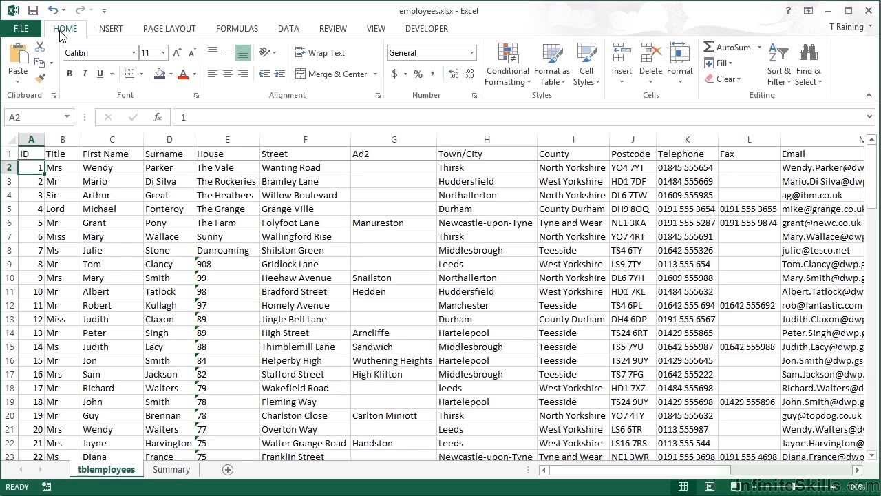
This will return the amount of the worths within a desired series of cells that all satisfy one requirement. For instance, =SUMIF(C 3: C 12,"> 70,000") would return the amount of worths in between cells C 3 and also C 12 from just the cells that are better than 70,000. Allow's claim you intend to figure out the earnings you generated from a list of leads who are connected with details location codes, or calculate the sum of specific workers' incomes-- however just if they drop over a particular amount.

With the SUMIF function, it doesn't need to be-- you can quickly build up the sum of cells that meet specific criteria, like in the salary example over. The formula: =SUMIF(range, criteria, [sum_range] Variety: The range that is being checked using your standards. Standards: The requirements that establish which cells in Criteria_range 1 will certainly be included with each other [Sum_range]: An optional series of cells you're mosting likely to accumulate along with the first Array went into.

In the example listed below, we intended to determine the amount of the wages that were more than $70,000. The SUMIF function accumulated the buck quantities that surpassed that number in the cells C 3 through C 12, with the formula =SUMIF(C 3: C 12,"> 70,000"). The TRIM formula in Excel is represented =TRIM(text).

All About Excel If Formula

For instance, if A 2 includes the name" Steve Peterson" with unwanted rooms before the first name, =TRIM(A 2) would certainly return "Steve Peterson" without spaces in a brand-new cell. Email and also file sharing are terrific tools in today's office. That is, till among your coworkers sends you a worksheet with some really cool spacing.

As opposed to painstakingly removing as well as adding rooms as required, you can clean up any type of uneven spacing utilizing the TRIM feature, which is used to get rid of added areas from information (except for solitary areas between words). The formula: =TRIM(message). Text: The text or cell where you desire to remove areas.

To do so, we got in =TRIM("A 2") right into the Formula Bar, and also duplicated this for each name below it in a new column alongside the column with undesirable spaces. Below are some other Excel solutions you may find helpful as your information monitoring requires expand. Allow's say you have a line of message within a cell that you wish to break down right into a few various segments.

Purpose: Used to remove the first X numbers or personalities in a cell. The formula: =LEFT(text, number_of_characters) Text: The string that you wish to draw out from. Number_of_characters: The number of personalities that you desire to draw out beginning with the left-most personality. In the instance listed below, we went into =LEFT(A 2,4) into cell B 2, and duplicated it right into B 3: B 6.

Purpose: Used to extract personalities or numbers between based upon placement. The formula: =MID(text, start_position, number_of_characters) Text: The string that you desire to extract from. Start_position: The placement in the string that you desire to begin drawing out from. As an example, the first setting in the string is 1.

The Of Excel Shortcuts

In this example, we entered =MID(A 2,5,2) into cell B 2, and also replicated it into B 3: B 6. That allowed us to remove the two numbers starting in the 5th position of the code. Objective: Made use of to remove the last X numbers or personalities in a cell. The formula: =RIGHT(message, number_of_characters) Text: The string that you wish to remove from.

formulas excel tutorial excel formulas list download formula excel mod